
One of the fundamental ideas in machine learning is the concept of training a model. This process is fundamentally an approximation of the solution: starting with a randomly initialized model we iteratively adjust a model’s parameters until its predictions are “good enough.” By the end, the model has “learned” a set of parameters that minimize some chosen error metric. In practice, though, training can be incredibly costly, often requiring massive compute resources, long runtimes, and substantial engineering effort.
So it’s natural to ask a slightly rebellious question: Do we really need training at all?
Could there be a silver bullet, a single analytical equation that takes a dataset (X,Y) and directly spits out the optimal model parameters? No iterations, no hyperparameter tuning, no trial and error. Just plug in the data and get the answer.
At first glance, this might seem like a strange question. After all, nearly every machine learning method today depends on iterative optimization. But that assumption is worth challenging. What we’re really asking is whether a closed-form solution exists — an explicit formula that gives us the optimal parameters directly, without any need for a search.
Before we dive in, let us first refresh the basics and make the goal concrete.
Assume you’re given a dataset represented compactly in matrix form, with input features X and corresponding labels Y. A supervised machine learning (ML) model aims to learn a mapping f(X) → Y. In other words, we want a function that describes the relationship between the input and the output. The form of this function or relationship is mostly arbitrary, but a common starting point is to just encode it as an unknown matrix, call it A. Thus, we can write f(A) as:
Or equivalently
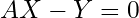
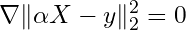
The hope is that this matrix A captures the underlying relationship between inputs and outputs. Of course, in most cases, no matrix A exists that satisfies AX = Y exactly. This is a fact from basic linear algebra: unless Y lies in the column space of X, an exact solution is impossible. Okay fine, maybe no matrix exists to satisfy the condition exactly (which is the case most of the time). But maybe we can talk about some error metric, or some notion of ‘’distance” away from 0. If no A exists such that I can exactly satisfy the 0 condition, maybe I can relax the requirement and opt to find a matrix that is very, very, very close to 0 somehow. This naturally leads us to define a norm (typically the squared L2 norm for vectors or the squared Frobenius norm for matrices). We can rewrite the problem as:

This reframing allows us to restate the problem in simpler terms: instead of asking for a perfect solution, we now ask for the one that is closest to perfect. In other words, we are no longer demanding that AX = Y exactly. We are instead asking for the matrix A that makes the difference AX-Y as small as possible (where 0 is the lower bound of that metric). If an exact solution does exist for A, then minimizing the distance ‖AX−Y‖ will naturally recover it. This follows directly from the basic properties of norms
This shift is crucial. Once we start thinking in terms of distance, the problem becomes well-defined even when perfection is impossible. We are no longer asking for zero error; we are asking for the smallest possible error.

Congratulations, we’ve just defined the fundamental problem underlying all of machine learning: at its core, it’s simply an optimization problem. (Here I am making no assumption on the real structure of A yet, but for the sake of argument just assume it’s some unknown quantity I need to find) The central question now becomes: how do we actually find A? In essence, this is a search problem. And this is precisely what we’re asking when we wonder whether closed-form solutions exist for neural networks.
Usually solving this problem entails using a standard iterative optimization process called gradient descent (GD). GD is essentially what “training” refers to. Training a model, in this sense, is nothing more than repeatedly adjusting A to reduce the loss, step by step, until further improvements become negligible.
The issue, of course, is that this process can be slow, expensive, and sensitive to many factors, especially when X, Y, or A are large. Which brings us back to the original question motivating this discussion: does a closed-form solution exist? Is there a direct formula that allows us to plug in X and Y and immediately recover the optimal A, without doing GD?
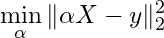
When facing a complex problem, a good first step is to simplify the setting. In our case, that means starting with the linear model. Here, let us reduce the matrix A to a linear vector α, and the output Y becomes a vector y.
This simplification brings us to familiar territory: linear regression. For convenience, let’s define the objective function as f(α):
By making this restriction, we dramatically simplify the problem. We are no longer searching over a possibly arbitrary space of functions, but over a very specific and well-behaved class. In fact, the resulting objective has a particularly nice geometric structure: it forms a bowl-shaped surface. In mathematical terms we say the objective function is convex.
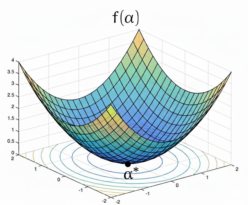
The best part about a convex function is that we know it has a single minimizer, which is essentially the bottom of that bowl. And guess what, the bottom of that bowl has a nice property that is very useful to us. The gradient at that point is equal to 0. This observation is crucial. If we know we have a single minimizer, and we also know that the gradient is 0 only at that minimization point, then we have a very easy and straightforward way of finding that point.
Just take the gradient of the objective (w.r.t α), set it equal to zero, and solve. No iterative search is required. No trial-and-error. Just algebra.
Solve for α:
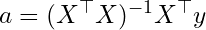
This gives us a closed-form solution for α, and if you have taken an introductory statistics course, the result will look very familiar. It is precisely the ordinary least squares (OLS) solution. For any given X and y, we can plug them directly into this expression and immediately recover the optimal parameters. Of course, this elegance comes with caveats. The matrix (X^⊤X) must be invertible, and even when it is, computing that inverse can be expensive for large-scale problems. In practice, these limitations matter. But conceptually, this is still a beautiful result: an exact, non-iterative solution that requires no tuning, no randomness, and no optimization heuristics.
Okay, so we were able to obtain a closed-form solution for a basic ML model, but notice the fundamental problem we had to solve: ∇f(α) = 0. Does this look familiar? What we are doing here is essentially the same thing the Babylonians used to do on clay tables, finding the roots of an equation. In their case, it was solving polynomial equations of the form P(x)=0. Here, the objective looks different, but the idea is exactly the same. Instead of solving for the roots of a polynomial, we are solving for the roots of the gradient function. That is, we are looking for values of α such that ∇f(α) = 0. So in this sense, OLS is nothing more than a root-finding problem. We are simply finding the point where the gradient vanishes.
So now we can make our question very precise. Let us return to the main question we started with: do neural networks admit such solutions? In other words, does there exist an analytical expression that characterizes the roots of the gradient function of a neural network’s loss? For linear regression, the answer is yes — we have an explicit, closed-form solution. But can we expect the same for neural networks? At a high level, the key difference lies in the structure of the model itself. In linear regression, the parameter vector α appears linearly, and the model can be written as a simple matrix–vector product. In contrast, a neural network replaces this linear structure with a composition of nonlinear functions. The “matrix” A is no longer a matrix in the usual sense — it is a nested composition of parameterized transformations. For example, the output of a 1 hidden layer NN looks like this W₂⋅σ(W₁(.)), where σ(.) is just the activation function. So now our optimization problem becomes
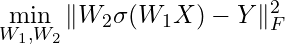
Then solving for an exact solution of the neural network essentially boils down to solving

Again, it might not look like it at first, but fundamentally we are still dealing with the same kind of problem we were dealing with in high school. We are trying to find the roots of an equation.
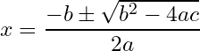
In the case of polynomials, root-finding is much more approachable. It’s one of the first major problem types introduced in basic math curriculums, and for good reason. In many ways, it represents one of the first major breakthroughs of modern mathematics beyond what was known in ancient times. The most familiar example is the quadratic formula, which provides an explicit solution for second-degree polynomials
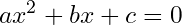
Where x can be found by just plugging in the values
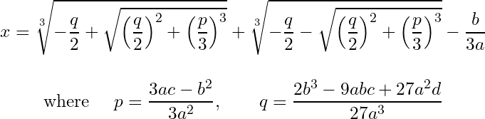
Surpassing this solution was given by Tartaglia and Cardano’s solution for the cubic polynomial.

The backstory behind the solution to the cubic equation is probably one of the most fascinating and scandalous in the history of mathematics. One could easily make an entire movie out of it (I highly recommend reading more about it here if you’re interested). That said, the solution is given by:
Turns out there’s an even uglier solution for the 4th degree polynomial that I will refrain from putting here but you can find it on Wikipedia.
But the quintic, 5th degree, polynomial is where we are going.

Évariste Galois was a young French mathematician who, at just the age of 18, proved one of the most remarkable results in mathematics. There’s a collection of theorems and definitions by Galois, showing a deep connection between field theory (‘fields’ as in, a vector space has vectors over a field) and groups (as in, a set of elements with a binary operation, an identity element, and a unique inverse to ‘undo’ any element feeding into the binary operation). One of the striking implications of Galois’ work is that if a closed-form solution exists for the roots of a quintic polynomial, then a very specific type of permutation group must also exist, one that captures the symmetries of the equation’s roots. But for quintic (and higher-degree) polynomials, this group turns out to be so complex (or "exotic") that it simply cannot exist. This insight proved that, in general, there is no closed-form solution for polynomials of degree five or higher. Galois unfortunately had a very sad ending to his math career. At just the age of 20 he died from wounds sustained in a duel, ending one of the most brilliant and promising mathematical careers in history.

So while the gradient function of a neural network isn’t exactly a polynomial, it lives in an even more intricate world: a deeply nested composition of nonlinear operations whose structure is vastly more complex than the algebraic equations. But think back to what Galois showed: even for a relatively simple, single-variable polynomial, like a quintic, the equation p(x)=0 can provably lack a closed-form solution. That insight should give us pause. If even a basic one-dimensional polynomial can defy exact solutions, is it really surprising that the gradient equations of deep neural networks — with their layers of nonlinearity and high-dimensional parameter spaces — don’t admit closed-form answers either? Neural network gradients may not be literal polynomials, but they share a critical trait: their root-finding problems quickly surpass the expressive power of algebraic methods. In short, solving them exactly with a neat equation isn’t just hard, in most cases it’s fundamentally impossible.
The problem here has nothing to do with non-convexity either. I can easily construct a non-convex function that still garners a closed-form solution. Here is an easy example

There are 3 critical points here. x ∈ {0, ± 1/sqrt(2)}. So just because the problem is non-convex doesn’t say much. Neural networks are nonlinear, coupled, and very high dimensional. Using basic arithmetic operations to get back a compact exact solution is unrealistic.
Another illustrative example is logistic regression. Despite being a convex problem, logistic regression does not admit a closed-form solution. To appreciate why, try this easy exercise: write down the loss function for logistic regression, take its derivative with respect to the learnable parameters, and attempt to solve for the roots. You’ll quickly see that the difficulty arises from the nonlinearity introduced by the sigmoid function. Unlike linear regression, there are no clean algebraic manipulations that allow you to isolate the parameters. The presence of exponential terms makes it impossible to rearrange the equation into a neat, closed-form solution. Approximations via algorithms like GD, in this case, are not optional but the only path forward. And here’s the kicker: the very idea behind Newton’s method (essentially second-order optimization) was developed and used by Newton himself to tackle the task of finding the roots of complex polynomials. Even he recognized that, for some equations, finding exact roots was either intractable or outright impossible — forcing us to rely on approximation techniques. It’s a bit poetic, really. The technological leaps we’ve made hundreds of years later still hinge on the same core challenges — and the same types of solutions — they faced in the 17th century. Nothing is truly new under the sun.
But poetic parallels aside, there’s also a very practical concern to keep in mind: the computational difficulty of the problems we’re dealing with. While convexity doesn’t determine whether a closed-form solution exists, it does play a critical role in the computational complexity of finding that solution. Just because something has a neat algebraic expression doesn’t mean it’s computationally cheap to evaluate. Take OLS as an example. It’s a convex problem and admits a clean, closed-form solution. But solving it is still expensive. The time complexity is O(n k² + k³), where n is the number of data points and k is the number of features. And if your matrix X is large, you’ll need sufficient GPU memory to carry out the matrix operations efficiently. In fact, OLS often requires more memory than gradient descent. So in practice, even when we have an exact solution, iterative methods like GD may be the more practical choice.
Now imagine — hypothetically — that a closed-form solution did magically exist for a neural network’s loss function. That wouldn’t necessarily make things easier. Neural networks are highly nonlinear and non-convex, and their loss landscapes can be extraordinarily complex. Evaluating such a solution, even if expressible analytically in principle, would likely be computationally intractable.

To illustrate this, suppose we somehow have a closed-form expression for the gradient function of a neural network’s loss: ∇f(W₂⋅σ(W₁)) = 0. Solving this equation gives us all the critical points, including local minima, saddle points, and possibly even maxima. But even after we solve this equation and pay the upfront computational complexity of obtaining the critical points, how do we know which of these points corresponds to the actual minimum of the loss function? In the convex case, it’s easy: the point where the gradient is zero is the global minimum. But for non-convex functions, this no longer holds. Every valley and every saddle point in the loss surface above corresponds to a zero gradient. That means even our magical hypothetical closed-form expression would still require us to examine each critical point individually to determine which one minimizes the loss. And with thousands or millions of parameters, the number of such points could be astronomically large. So even if we could write down a magical algebraic expression that solves for the roots of the gradient function, it wouldn’t help much. The challenge isn’t just in finding the roots — it’s in knowing what to do with them. In a landscape filled with deceptive critical points, closed-form analysis quickly becomes both computationally expensive and practically useless.
The difficulty of these problems is no coincidence. From the perspective of computational theory, non-convex optimization is NP-hard. So even if a closed-form solution for a neural network’s loss function somehow existed, it would likely be a tangled, computationally expensive mess. Worse, you’d still have to manually inspect every critical point it returns.
With all of this said, is it a surprise that our gradient equation has no closed-form solution where I somehow magically get the true minima? If it did, it’d be like instantly finding every single local minima that exists, all at once. If we had an equation that takes in latitude and longitude coordinates and outputs an altitude, we would instantly know all the mountains, hills, and valley bottoms on earth all at once, without actually having to fly around and look for them individually. But, just as with higher-degree polynomials, once you move beyond linear regression, you’re forced to rely on numerical methods. You don’t get a global map with every feature marked. You have to fly around the parameter space yourself, hill by hill, hoping you land near a good one. If you’re lucky, maybe your first stop is the tall peak you’re looking for.
So if you ever find an optimization problem that does have a closed-form solution, count yourself lucky. That’s the exception, not the rule. The number of problems that don’t have well-behaved solutions is shockingly larger than the number that do. Uncountably infinitely more. In a landscape filled with mathematical wilderness, the few gems we can solve directly are rare and precious.
As closing remark I want to give a credit to a random gem of a reply on Reddit by a user named adventuringraw. Their answer on a thread nudged me down this path, eventually leading to the deep dive and reflection that became this post.